
...they faced the prospect of performing frequency domain intra-prediction involving multiple, nonhomogeneous input and output block sizes. Aside from just being complicated, each possible combination would require its own set of prediction matrices, some quite large. The combinatorics alone render this scheme impractical. Wouldn't it be nice if they could change blocksizes by splitting blocks apart and merging blocks together? It would avoid the whole problem!
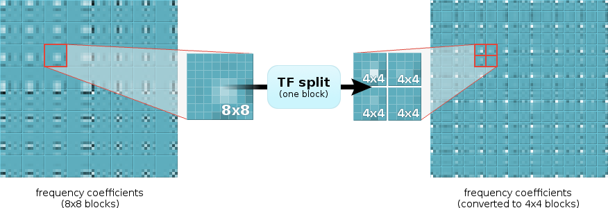
As it turns out, they ...ahem... we can! To escape certain death under a crushing mound of different blocksizes, we borrow a previous invention, Time/Frequency Resolution Switching ('TF' for short), from our Opus audio codec. TF allows us to split apart or merge together blocks while staying in the frequency domain. By altering the blocksizes, we can eliminate the nonhomogeneity and reduce both the size and number of required prediction matrices. For example, we could TF surrounding blocks to match the size of our input block, or always run prediction at a 4x4 blocksize.
TF is useful in a number of other places as well, so it's worth describing in some detail. Let's start by looking at what we want, what we really need, and then how TF delivers.
Obviously, we want TF to be as cheap to compute as possible. We'd like to avoid multiplies if possible, and reversing and re-computing the DCT for each blocksize is right out. It would also be nice if our transform showed uniform/unit scaling, minimal dynamic range expansion, and complete reversibility.
In short, what we really wish we could do is switch between multiple lapped blocksizes as if we'd done DCTs for every possible combination, and we want it for as close to free as possible. Not surprisingly, it turns out we can't get everything we want.
Our lapped transform uses a fast DCT, a member of the FFT family. All FFT-like transform structures begin with an initial 'butterfly' that operates pairwise on interleaved samples spread across the spatial input. Even though we can split most of a DCT in half down the middle of the input block, we can't split the first step. To merge two blocks or split blocks in half such that they're equivalent to the other transform size, we would in fact have to unwind all the way back to the spatial domain and recalculate the entire DCT.
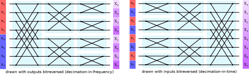
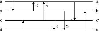
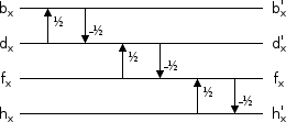
Figure 1: A simplified illustration of the butterflies in an eight-point FFT (leaving out the weighting factors). This underlying structure is the same whether the FFT is decimation-in-frequency, normally drawn with the inputs in ascending order, or decimation-in-time, normally drawn with the inputs bitreversed and the frequency coefficients in ascending order. Other transforms in the FFT family, such as the fast DCT, have a similar structure.
Regardless of how it's drawn, the butterflies in the first stage require inputs from both halves of the spatial input vector. We cannot split the original spatial vector 'in half' in the frequency domain without first reversing the entire process. Similarly, merging two blocks requires adding a new stage to the beginning of the computation, not end. As such, merging two spatial blocks in the frequency domain also requires first inverting the original FFT.
So, we can't split a DCT in half or merge two DCTs together without first unrolling them, and unrolling is too expensive. Even if we did, we'll run into lapping issues that still rob us of perfect victory. However we do this, we'll have to be satisfied with an approximation to the perfect TF transform we wish we could have.
To find this approximation, we ask ourselves "What are we really trying to do?" When we merge four blocks together into a single larger block, we're beginning with four neighboring frequency-domain blocks. These blocks may be frequency coefficients, but the relationship between coefficients in neighboring blocks is spatial. We want to transform that spatial relationship into the frequency domain. Splitting is the converse, converting a frequency relationship into a spatial relationship.
Ironically enough, we do this with a DCT! Taking four colocated frequency coefficients from neighboring blocks, a 2x2 forward DCT converts their spatial relationship into frequency. Similarly, taking a 2x2 block of frequency coefficients from a single block and using an inverse DCT, we convert their frequency relationship into a spatial relationship. The resulting output is not the same as recomputing the entire DCT of a different blocksize from scratch, but it does give us the frequency-domain approximation we're looking for— and the 2x2 case involves no multiplies.
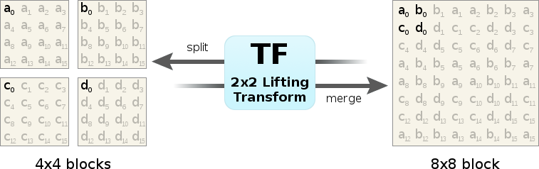
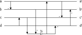
Figure 2: Frequency-domain blocks can be split or merged by iterative application of the 2x2 TF transform to groups of four frequency coefficients at a time. The diagram above shows the location of input and output coefficients in the source and destination blocks.
Note that coefficient ordering in the large block alternates in a folded pattern because the DCT is a symmetric (rather than circular) transform. An implementation can achieve the same effect by adjusting the signs of the coefficients of the small blocks rather than reordering the coefficients of the large block.
We also need a four-point transform to transform 4x4 blocks to 16x16 blocks and vice versa. Unfortunately, a four-point DCT requires multiplies. Of course, we could use a two-point DCT to transform from 4x4 to 8x8 and then use a two-point DCT again from 8x8 to 16x16. The resulting transform isn't a DCT though; it's a Walsh-Hadamard Transform (WHT).
Technically, the two-point DCT and WHT (and Haar Wavelet Transform for that matter) are equivalent. As we've just noted, you can't build a larger DCT by stacking smaller DCTs. However, stacking two identical Walsh-Hadamard transforms does result in a WHT of twice the size. Since the two-point cases are the same, that's why our stacked 2x2 'DCT' magically transformed into a 4x4 WHT.
As transform size increases, the WHT remains cheap to compute (no multiplies). In Daala, of course, we need only the 2x2 and 4x4 WHT.

| "We're in zero-G. How do you keep your coffee cup on the table?" |
| "Velcro." |
| "What about the coffee?" |
| "More Velcro!" |
| —Mark Stanley, Freefall |
The remaining properties on our wishlist are unit/uniform scaling (all outputs are scaled by a factor of 1), minimal range expansion, and exact reversibility in an integer implementation. We used lifting filters before to implement a lapped transform with these properties, so we'll use more lifting to do the same for TF. This is a bit low-level, but it's fun to walk through the logic of designing the lifts.
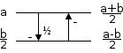
Our 2x2 transform is pretty simple. The dimensions are separable, so we can run a 2 point WHT on the rows, and then run it again on the columns. The basis functions for the two point WHT are [1,1] and [1,-1], scaled as we see appropriate. So we do the obvious thing; design a lift that computes the outputs as [a+b, a-b]:
lifting pseudocode:
b := a - b;
a := (2*a) - b;

It's simple and gives the right answer. Of course, it has an obvious problem; the output is scaled up by a factor of √2 with each step. After we stack them, the final 2x2 transform's output will be scaled up by a factor of two and the dynamic range quadrupled.
We can't simply shift down both outputs at the end, and scaling each leg by √.5 involves multiplications. We'll need to find some other way to build a lifting stage that doesn't scale the output. Here's another attempt:
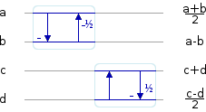
lifting pseudocode:
b := a - b;
a := a - (b/2);

This achieves the goal of not scaling the overall output, but now the output scaling isn't uniform. The upper leg's output is scaled by half relative to the lower leg. This is the choice we appear to be stuck with: the outputs being scaled up, or output scale asymmetry.
If we play with the asymmetric scaling choice a bit longer, we'll notice we can swap the relative scaling asymmetry between outputs by shifting operations around. Compare:
lifting pseudocode:
a := a + b;
b := (a/2) - b;

We can also push the asymmetry to the other side and design lifting stages that take asymmetrically scaled inputs and produce symmetrically scaled outputs:
lifting pseudocode:
a := a + (b/2);
b := a - b;

lifting pseudocode:
b := (a/2) - b;
a := a - b;
At this point, we have a little collection of four asymmetric lifting stages. Each reversibly computes a 2 point WHT without scaling the overall output, but the individual outputs/inputs are asymmetrically scaled relative to each other. Then we realize these asymmetries are all complementary!
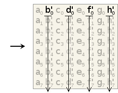
Since the starting inputs are implicitly symmetrically scaled, we start the 2x2 transform using the lifting stages that expect symmetric inputs. The first transform applies to the even column, and the second to the odd column. This produces asymmetrically scaled intermediate values:

Then we can use the stages that expect asymmetrically scaled inputs to transform the columns:

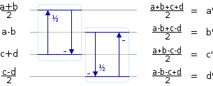
String it all together, and we have a complete 2x2 WHT transform:
lifting pseudocode:
b := a - b;
a := a - (b/2);
c := c + d;
d := (c/2) - d;
a := a + (c/2);
c := a - c;
d := (b/2) - d;
b := b - d;

Some easy transformations get the operation count down to seven adds and one shift per four pixels if we use an extra register. Starting by reordering the operations:
lifting pseudocode:
b := a - b;
c := c + d;
a := a - (b/2);
a := a + (c/2);
d := (c/2) - d;
d := (b/2) - d;
c := a - c;
b := b - d;
Alter the signs and ordering around d to eliminate the successive negations:
lifting pseudocode:
b := a - b;
c := c + d;
a := a - (b/2);
a := a + (c/2);
d := d + (b/2);
d := d - (c/2);
c := a - c;
b := b - d;

And now we see that we can arithmetically collapse several operations if we use an extra register, e:
lifting pseudocode:
b := a - b;
c := c + d;
e := (c - b)/2;
a := a + e;
d := d - e;
c := a - c;
b := b - d;
And with that, we have a fast, reversible 2x2 WHT with unit scaling, the minimum possible range expansion (doubled), and no multiplies. It has one other useful quirk— it's its own bit-exact reverse. We don't even need to implement an inverted version. And, of course, we can use this exact same filter implementation to split blocks as well as merge them.
Note that this is not the only possible implementation. We can shuffle the asymmetries and sequence of operations to implement versions with slightly different integer rounding behavior. The implementation shown here matches the Daala source as of August 2, 2013. We submitted this WHT plus a few variants to Google for use in VP9's lossless coding mode; they chose one of the alternate versions of the WHT illustrated above.
TF as we've implemented above is a very-cheap-to-compute approximation of the transform we were actually aiming for: a true DCT of the alternate blocksize. How good is this approximation?
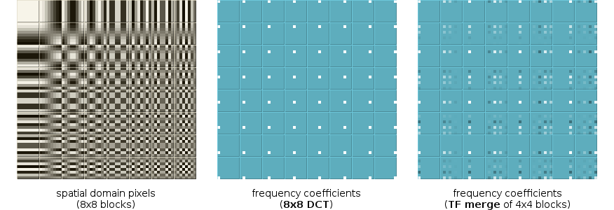
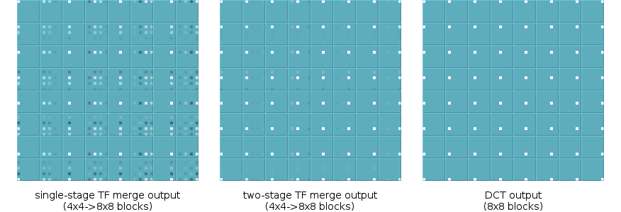
Let's use something easy to see: transformed basis functions. We start with a grid of 4x4 blocks, with alternating blocks containing one of the 4x4 DCT basis functions. We transform each block into the frequency domain with a 4x4 DCT. The output blocks contain a single non-zero frequency coefficient each, confirmation that our inputs are basis functions. This is the ideal 4x4 output that we'll compare to 4x4 blocks we manufacture using TF splitting.
Now we start with the same input values, but grouped together into larger 8x8 blocks. We transform them to the frequency domain using 8x8 DCTs; note that the frequency domain looks quite different:

Finally we split each 8x8 frequency domain block into four 4x4 blocks using TF. Compare the 4x4 TF output to the output produced directly by the 4x4 DCT (two diagrams above).
Let's also compare TF merging using a similar process. We begin this time with the 8x8 DCT basis functions, so that our ideal 8x8 frequency-domain blocks contain one nonzero frequency coefficient each. Skipping straight to the results:
Neither the split nor the merge are that bad of an approximation for such a cheap transform... but we notice something in the TF-merge results. There's an obvious pattern to the output error that's partly position-invariant with respect to the nonzero coefficient.
Earlier, I said that different DCT transform sizes differ in the number of stages at the beginning (not end) of the transform, and so there's no way to alter the transformed blocksize of a DCT without first completely undoing the DCT. That's not quite true; we can change the blocksize of a DCT after the fact, but it theoretically requires N^2 operations. Completely recomputing the DCT is cheaper.
However, the error pattern in the TF-merged output suggests we can improve our cheap approximation, and in fact we can. A simple secondary lifting filter applied to the rows and then columns of the initial TF output block improves the mean squared error by more than an order of magnitude:


We build a two-stage TF split transform as expected; use the inverse of the second stage filter as a prefilter to the one-stage splitting transform. The additional filter stage improves splitting as much as it improves merging.
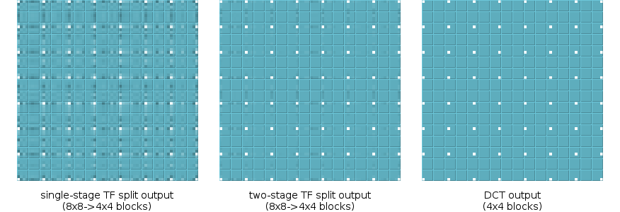
We can continue improving the filter to come arbitrarily close to the exact DCT output if we want. For example, six additional add/shift operations can further reduce output error by half. However, the cost of larger filters yields steeply diminishing returns.
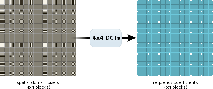
We've spent this whole time looking at transformed basis functions, mainly because the sparse frequency domain makes error very easy to see. Below, we see TF merge/split used as an approximation to the DCT, as applied to a real image. This is only a single image example, but the results are representative of general behavior.

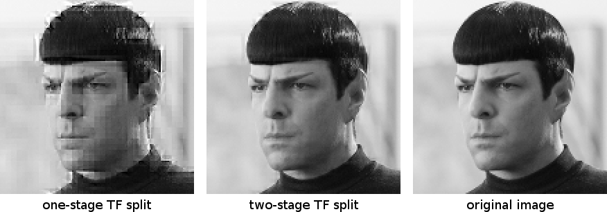
There's a glaring 'error' in all of the above TF work: we've been modeling performance of the DCT, not our lapped transform. Single-stage TF using a WHT is a rough enough approximation that lapped or not makes relatively little difference. However, the second TF stage dramatically improves results, and it's possible that it could be (and should be) tuned to our lapped transform rather than the DCT.
We also shouldn't forget that TF isn't just low-cost, it's a reversible transform. Our new-and-improved TF, or a variant of it, may show sufficient coding gain that we could potentially use it to replace larger DCT blocksizes entirely. In one possible scenario, we'd transform everything as a 4x4 lapped transform and build larger blocksizes from TF. That would increase speed and solve all our various heterogeneous blocksize problems-- if it actually works.
Call that future research for now.
There's also still quite a bit to cover in the overall Daala design. Next demo, I think we'll look at another place we use TF: Predicting the Chroma planes from the Luma plane (page now up!).
—Monty (monty@xiph.org) August 12, 2013