Contrary to the standard presentation, we first define the Euclidean Distance Transform in a continuous domain, and then discuss how that definition can be adapted to work with binary images defined over a discrete domain. We show how the standard definition leads to discrete signed distance transforms which cannot be produced by any underlying continuous domain shape. This is clearly worrying when working with digital images that are meant to be discrete representations of real-world objects in a continuous domain. We present an alternative definition which preserves the important property of inverse-consistency from the continuous domain definition and which guarantees that any discrete domain shape has an underlying continuous domain shape that produces the same signed distance transform.
Let S ⊆ ℝd be a d-dimensional shape and define a binary image I of S as the characteristic function of S:
| I : x ∈ℝd → χS(x) , |
where χS(x) is 1 whenever x ∈S, and 0 otherwise. Then the Euclidean Distance Transform (EDT) of I is defined as
| EI : y ∈ℝd → | inf | ∥y - x∥ . |
| x ∈S |
Intuitively this transform represents the distance to the closest point in the shape. It has numerous practical applications in the fields of pattern recognition, shape analysis, and robotics, and medical image analysis [Pagl92,Cuis99]. The use of the infimum in the definition ensures that boundary points are treated the same, regardless of whether the appear in the shape or in the background. Although this definition is simple in the continuous domain, consistency problems emerge with typical methods of restricting the domain of x to a regular grid.
These problems are most directly exhibited by the signed distance transform, which is an extension of the original definition to include a negative distance to the background in the interior of the shape1. More formally, let 1-I be the binary image of SC, the complement of S. The signed distance transform is then defined by the distance transform of both the original shape, S, and of the background, SC:
| GI(y) =EI(y) - E(1-I)(y) . |
It is easy to see that this definition is inverse-consistent: G(1-I)(y) = -GI(y) . This implies that the definition is symmetric with respect to what is the foreground shape and what is the background. It ensures the magnitude of the gradient is one everywhere, except at points on the medial axis (of either the shape or the background), where no single gradient is defined. The boundary of the shape is given by the 0 level set of G.
Computer images are typically defined in a discrete, not continuous, domain. There are several ways to modify the definition to work with a discretely sampled image. Ultimately these all boil down to defining what image over the continuous domain is implied by its discretely sampled version.
Let Î be the discretely sampled version of I:
| Î : x ∈ℤd → I(x) . |
One can recover a discretely sampled version of the shape, Ŝ, from Î via
| Ŝ = { x ∈ℤd : Î(x) = 1 } . |
Then, supposing there is some way to recover a continuous shape S (and thus I) from Ŝ, the discretely sampled version of the distance transform, Ê, is given by
| ÊÎ : y ∈ℤd → EI(y) . |
There are now at least two ways to define a signed transform. One is to pull back the signed transform from the underlying continuous shape:
| ĜPBÎ : y ∈ℤd → GI(y) . |
The other is to enforce inverse-consistency directly in the discrete domain:
| ĜICÎ : y ∈ℤd → ÊÎ(y) - Ê(1-Î)(y) . |
Both ways require a method of recovering S from Ŝ.
One choice is to use Ŝ directly in the inverse-consistent definition:
| ĜDÎ = ĜICÎ , S = Ŝ . |
This is equivalent to just replacing ℝd with ℤd in our original definition of E:
| ÊDÎ : y ∈ℤd → | min | ∥y - x∥ . |
| x ∈Ŝ |
This direct method is the classical way of defining the unsigned transform for discrete binary images. Under this view, the image Î represents an underlying constellation of lattice points, not (one or more) non-trivial, connected objects. However, using Ŝ directly in the pull-back definition does not produce consistent results: because SC contains all of ℝd except a countable number of isolated points, E(1-I) is zero everywhere and thus GI is non-negative everywhere. Furthermore, there is no general construction of S for which Ê = ÊD and ĜPB = ĜIC . Any point in Ŝ that has a 2d-connected neighbor not in Ŝ produces two adjacent lattice points with ĜIC values of 1 and -1. However, if ĜPB produces the same values, this implies one point is contained in an open ball of radius one inside S and the other is contained in an open ball of radius one inside SC. These two balls intersect, generating a contradiction. This explains why this direct extension of the continuous definition is never used in practice for the signed transform.
Grevera proposes treating all such border elements as lying at distance 0 instead of ±1, both immediately inside and immediately outside the shape [Grev04]. This produces a distance which is symmetric, and which could in theory be generated by a continuous domain set S, but requires a construction where, for example, both interior and exterior points are dense in the space between these pixels. This does not have a natural correspondence to real-world objects, but they note that with a simple modification, their method becomes equivalent to the morphological method described below.
A number of authors take a non-symmetric approach designed to eliminate the simple counter-example presented above [Dani80,Grev04,TSG06]. The idea is to construct a background image Ĵ not by taking the set complement of Ŝ, but by performing a morphological dilation on (1-I) using a closed ball of radius 1 as the structuring element2. That is, let
| Br | : x ∈ℤd → { y ∈ℤd :∥y - x∥≤ r } | ||
| Ĉ | = ŜC ⊕ B1 = | ⋃ | B1(z) |
| z∈ŜC | |||
| Ĵ | : x ∈ℤd → χĈ(x) . | ||
Then,
| ĜMÎ : y ∈ℤd → ÊDÎ(y) - ÊDĴ(y) . |
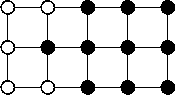
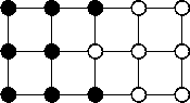
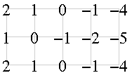
The results are better than those of the direct method. A boundary is established where the foreground and background images intersect, ensuring that ĜMÎ is zero on this boundary and has a magnitude no larger than one at its 2d-connected neighbors. Hence our previous counter-example no longer holds. But even with this alternative, non-symmetric definition of an "inverse", we can still find an example where the distances returned cannot be generated by any set S in the continuous domain. Consider the example in Figure 1.
|
|
|
| (a) | (b) | (c) |
| Figure 1: An example of a distance transform computed by the morphological method that cannot be obtained by an underlying shape S in the continuous domain. (a) A section of the foreground image, Î. Open circles represent zeros and filled circles represent ones. (b) The corresponding section of the background image, Ĵ. (c) The resulting signed distance transform, ĜM. We have left the magnitudes squared here so that they are still integers. | ||
The center pixel where ĜMÎ = -1 has two neighbors where ĜMÎ = 1 that are only √2 away. Hence, there is an open ball of radius one which must be in S which intersects with two other open balls of radius one which must be in SC, leading to another contradiction. A similar construction can be produced for d = 3 .
This note proposes an alternative method of computing a discrete signed distance transform that is both inverse-consistent and corresponds directly to an underlying continuous representation. We define that underlying representation by construction. Let P(x) be a closed box in ℝd of diameter 1 centered around x. That is,
| P : x ∈ℝd → { y ∈ℝd : ∥y - x∥1 ≤ ½ } , |
| S : Ŝ ∈𝒫(ℤd) → | ⋃ | P(z) , |
| z ∈Ŝ |
where 𝒫(·) is the power set. It is easy to see that S(ŜC) is just the closure of S(Ŝ)C, and hence this definition is inverse-consistent. That is,
| ĜTÎ = ĜPBÎ = ĜICÎ , S = S(Ŝ) . |
It is relatively easy to compute ĜTÎ according to this definition by finding the distance to the shape boundary. The morphological method computes a shape boundary as the intersection of Î and Ĵ. If these isolated pixels are replaced by a connected curve that passes through them, then for some pixels in the result the closest point on the curve does not lie on the grid. In our method, the boundary always lies halfway between two grid positions. If we double the grid resolution, we can sample this boundary directly. However, because our boundary never moves diagonally, as that in Figure 1 does, the closest boundary point always lies at an upsampled grid location. Therefore, the direct method applied to this boundary image produces the correct magnitudes at the original grid locations. Downsampling the result and negating the values inside Ŝ produces the desired ĜTÎ.
In practice, there is no need to compute the boundary image explicitly, which has complexity and storage requirements of O(2dn), where n is the number of input pixels. Instead, ĜTÎ can be computed directly from the original image using a modification of Felzenszwalb and Huttenlocher's O(dn) algorithm for computing ÊDÎ [FH04]. This is slightly more complex the original algorithm, but only by a constant factor. In practice it runs about 29% slower.
Example code is given in edt.c. It should build on any Unix system with
make edt
(no Makefile required), or on other platforms with the compiler of your choice. The code is restricted to two-dimensional images, but a generalization to higher dimensions is straightforward. It takes as input an image height and width, followed by an appropriate number of zeros and ones, and outputs both ĜTÎ and ÊDÎ . Both output squared magnitudes, with the former in quarter-pel units, to allow exact integer arithmetic to be used. Example input can be found in edt.in, with the corresponding output in edt.out.
1Note that this is not the "signed" distance transform referred to by Cuisenaire [Cuis99]. The latter does not produce a distance at all but a vector pointing to the closest point in the shape. That is more commonly called the closest feature transform (FT), e.g., by Maurer et al. [MQR03].
2The exact shape of the structuring element only matters for non-isotropic grids, a case which for simplicity we are not considering here. In an isotropic grid, such a ball simply contains a pixel and its 2d-connected neighbors.
| Comments or questions? Send them to tterribe@xiph.org | Created 15 Dec. 2007, last updated 22 Dec. 2007 |